

Nine case studies, one end-to-end workflow
Setup, labels, features, models, costs, risk — what the ML4T strategy research workflow does at every stage.

The early chapters of Machine Learning for Trading, 3rd edition, introduce a research workflow for systematic strategy development. Chapters 6 through 20 then apply it to nine case studies that span seven asset classes, five forecasting horizons, and frequencies from 8-hourly to monthly. The case studies are concrete, worked examples a reader can pick from — the one closest to your data, cadence, or asset class. This issue walks through what the workflow does at each stage, with pointers to where the libraries that support it are located.
Each case has its own page at ml4trading.io/case-studies with pipeline details, related chapters, and links to the GitHub code.
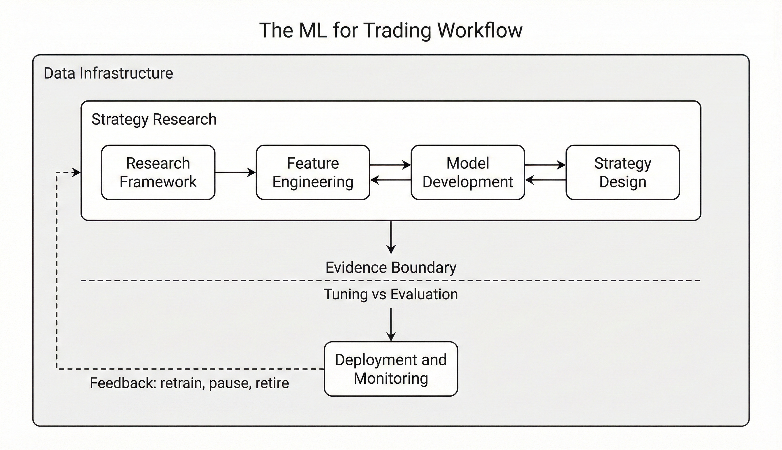
The ML for Trading workflow that organizes the book — research loop above the evidence boundary, deployment below, and feedback closing the cycle.
What the workflow does at each stage
Setup (Chapter 6). Each case begins with an explicit specification: the asset universe, the rebalance cadence, the train/validation/holdout split, the baseline checkpoints the case will measure itself against, and a search-accounting log that records every model trained — feature inputs, hyperparameters, fold-level metrics, and runtime artifacts. Chapter 6 argues for explicit search accounting as a guard against backtest overfitting: reproducibility is hard to recover once prior runs have disappeared from memory.
Labels (Chapter 7). The label is the quantity the model is trained to predict; defining it is a modeling decision, not a downstream encoding of a separate target. Chapter 7 organizes labels into fixed-horizon and variable-horizon families. Fixed-horizon labels are evaluated at a predetermined offset: continuous forward returns over the trading horizon for regression, or discrete state codes — the sign of the return, a quantile bucket, or exceedance of a volatility-scaled threshold — for classification. Variable-horizon labels let the realized horizon depend on the path: trend-scanning labels expand the look-forward window until a trend test rejects, and triple-barrier labels resolve when one of a profit target, stop loss, or time limit binds first. Horizon and the instrument’s cost regime at that horizon constrain the choice — a 21-day forward return on monthly ETFs is a different estimation problem than an 8-hour funding-period return on crypto perpetuals. Label construction primitives, alternative bar samplers, and the overlap-aware sample-weighting they require are provided by ml4t-engineer.
Features (Chapter 8). Engineered features come from ml4t-engineer: roughly 120 technical indicators across 11 categories — momentum, volatility, trend, volume, microstructure, and others — Polars-native and JIT-compiled, with around 60 cross-validated against TA-Lib. Where the asset structure supports them, alternative bar samplers (volume bars, dollar bars, tick-imbalance bars) replace fixed-time bars; microstructure features appear when intrabar data are available.
Model-based features (Chapter 9). Features extracted from auxiliary statistical models fit per series, used to encode dynamics that engineered indicators capture only loosely:
Kalman-filtered states and innovations,
spectral and path-signature coefficients,
ARIMA residuals,
GARCH and HAR/rough-volatility estimates,
HMM and Wasserstein regime posteriors,
fractional-differencing transforms for stationarity, and
uncertainty-aware variants of each.
The distinction is mechanical rather than thematic — the feature is an estimated quantity from a fitted model, so its training-time and inference-time computation has to respect the same purged-walk-forward discipline as the prediction model that consumes it.
Feature evaluation (Chapter 7, second pass). Before any model is trained, every feature is screened individually — daily cross-sectional information coefficient, ICIR, HAC-robust standard errors, walk-forward folds. Features that fail the triage screen do not silently carry forward into model training. The diagnostic machinery here lives in ml4t-diagnostic, which also provides the deflated Sharpe ratio, combinatorial purged cross-validation, and the multiple-testing corrections used downstream.
Model families (Chapters 11–15). Each case runs the families that fit its data:
regularized linear models (Chapter 11),
gradient-boosted trees and tabular deep learning (Chapter 12),
sequence deep learning, including LSTMs, TCNs, and transformers ( Chapter 13),
latent-factor models, including IPCA and a stochastic-discount-factor specification (Chapter 14), and
double machine learning for the cases where confounding is the open question (Chapter 15).
The latent-factor and SDF estimators, together with a conditional-autoencoder model and several end-to-end portfolio-learning architectures, are packaged in ml4t-models — the most recent of the six libraries. Hyperparameter search and fold-level evaluation are uniform across families; comparability across cases comes from running the same protocol everywhere, not from picking a per-case favorite.
Signal-stage backtest (Chapter 16). Predictions become positions through the backtester provided by ml4t-backtest — event-driven with point-in-time correctness, exit-first order processing matching real broker behavior, configurable same-bar or next-bar fills, and quote-aware execution that distinguishes bid, ask, and midpoint sources. The same code path runs the validation backtest and the frozen-holdout backtest, with no leakage between them.
Portfolio construction (Chapter 17). Allocator choice is part of the experiment. Equal-weight long-short top-N is the baseline; risk parity, mean-variance with shrinkage, and robust-optimization variants run alongside where the universe supports them. End-to-end portfolio-learning models — where the allocator is itself learned rather than rule-based — are part of ml4t-models. The point is to isolate how much of any net result comes from the signal and how much comes from the allocator.
Transaction costs (Chapter 18). Costs are modeled instrument-by-instrument and calibrated to the level a participant trading the case-study universe would incur, rather than a flat basis-point placeholder applied uniformly. Equity bid-ask half-spreads are derived from quote data with a bottom-quintile discipline; futures roll costs and continuous-contract artifacts are handled at the bar-construction level; FX uses interbank-spread approximations; option strategies use premium-scaled bid-asks sized to the round-trip; per-share commissions enter where the cadence makes them binding. Each case reports a sensitivity analysis at multiple cost levels — a single static cost assumption hides where the strategy actually breaks down. The cost machinery sits on the same execution layer as the backtester.
Risk overlays (Chapter 19). Daily-loss caps, drawdown-triggered position cuts, position-size limits, and regime-aware sizing where the data supports an explicit regime layer. The overlays are applied as a separate pass over the cost-aware backtest output rather than fused into the signal stage. Keeping them separate preserves a useful diagnostic distinction: when a result disappoints, you can ask whether the signal had alpha that the cost regime erased, whether the risk overlay was the binding constraint, or whether the overlay never engaged at all.
Cross-case analysis (Chapter 20). The synthesis appears in Chapter 20, which treats the nine cases as a single experiment rather than nine independent reports. It examines how well upstream feature-triage diagnostics predict downstream strategy survival, identifies, case by case, where prediction quality, portfolio translation, or execution friction is the binding constraint, and points to the lever each case suggests for the next research iteration. Detailed per-case numbers are the subject of upcoming issues.
What’s coming
Coming issues will move case-by-case — each case’s binding constraint, the iteration step the evidence suggests, what changed between research cycles, and the open questions left on the table. The cross-case synthesis from Chapter 20, individual stages worth a deep dive (feature triage, instrument-specific cost modeling, allocator comparison), and the methods themselves all have their own future issues queued up.
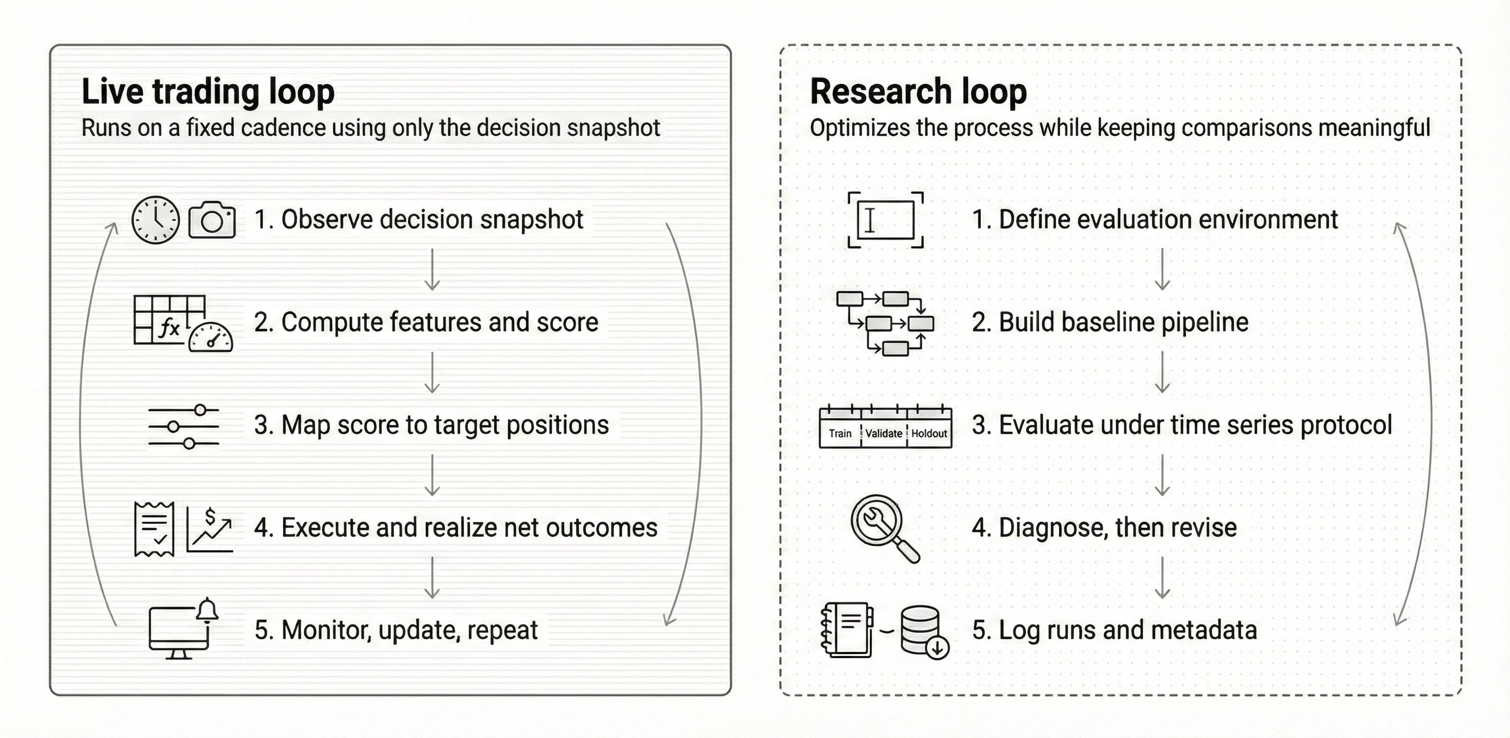
The research loop from Chapter 6, alongside the live-trading loop. The new case-study iteration agent runs inside the right-hand loop.
A new agent has also joined the research loop. It runs its own iterations on each case study — re-running setup decisions, refining the feature panel, adjusting cost assumptions and risk parameters, and proposing the next experiment to try. Whatever it surfaces worth reporting will land here.
Per-case detail lives at ml4trading.io/case-studies. GitHub repo going live close to launch.