New Release: The ML4T Data Layer Is Now Public

This release makes the Chapters 1-5 code public and focuses on the data foundation: data loaders, market microstructure, as well as alternative and synthetic data.

Today, we are releasing the code for the first five chapters of the third edition of Machine Learning for Trading.

Chapter 1, The Process Is Your Edge, sets up the workflow: define the research problem, keep exploration separate from confirmation, and treat live degradation as something the process has to handle. Chapters 2-5 then make the data foundation inspectable.

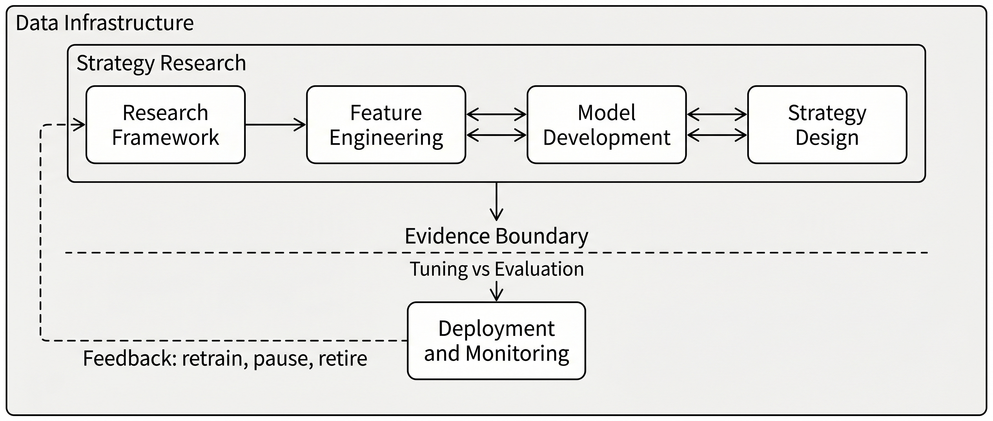
Data infrastructure supports strategy research and live deployment. This release provides access to the book's coverage of the infrastructure layer: the data and chapter notebooks that later case studies build on.

This release also arrives as we start teaching the ML4T workflow live. The free From trading idea to validated strategy Lightning Lesson runs Wednesday, June 24, at 16:00 UTC / noon ET; the full Machine Learning for Trading: From Research to Production course starts July 6. The course is organized around this loop: start with a research question, build the data contract, cross the evidence boundary only when the experiment deserves it, and carefully track the live feedback loop.

In trading research, few things are more important than the information contained in data, and how to handle it properly: clocks, sessions, adjustments, revisions, identifiers, contract rolls, venue rules, licensing limits, and the question of what a strategy could have known at the time of the decision. A later model result only means something once those choices are visible.

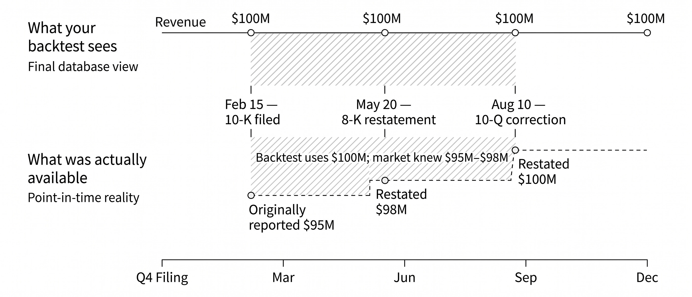
A point-in-time accounting example from Chapter 4. The final database view shows the same $100M revenue value across the year; the lower track shows what was actually available after the original filing and later restatements.

This release adds the first five chapter directories and the central data/ package that later case-study work builds on:

• Chapter 1: The Process Is Your Edge

• Chapter 2: The Financial Data Universe

• Chapter 3: Market Microstructure

• Chapter 4: Fundamental and Alternative Data

• Chapter 5: Synthetic Financial Data

• The data download package

Chapter 1 adds the workflow frame. The four data chapters contain 62 notebooks. The data/ directory adds the catalog, download scripts, loaders, configs, and access notes that turn the chapter examples into something a reader can inspect and run. The implementation detail worth checking first: loaders return Polars DataFrames through a consistent API, and missing data raises setup instructions with explicit download guidance.

What the data layer contains

The top-level data catalog currently lists 31 dataset entries. Financial data does not fit cleanly into one giant downloadable bundle. Some sources can be fetched without an API key. Some need a free key. Some are paid. Some require a manual provider download. Some reduced licensed packages are still being prepared for hosting.

The catalog groups entries around the constraints a research workflow inherits: daily market data, microstructure feeds, options data, fundamentals, positioning, macro series, prediction markets, on-chain metrics, news, and text. That structure makes setup expectations and redistribution limits visible before a reader spends time trying to reproduce a notebook.

The synthetic-data chapter takes a different angle. It asks how to create alternative histories for robustness analysis when one realized market path is not enough. The notebooks start with classical simulation and move through TimeGAN, Tail-GAN, Sig-CWGAN, GT-GAN, Diffusion-TS, LLM-based tabular generation, and differentially private GAN training. The diagnostics focus on stylized facts, dependence structure, downstream task utility, and privacy constraints.

Chapters 2-5 in one pass

Chapter 2 gives the map. It covers the financial data universe by asset class and source type, then moves into due diligence and storage. The practical thread is that provider data already contains research choices: corporate actions, survivorship, contract construction, point-in-time availability, storage format, and update policy.

Chapter 3 gets closer to the tape. Market data is the output of market design: sessions, order types, venue rules, visible liquidity, and timestamp conventions. The notebooks parse NASDAQ TotalView-ITCH, reconstruct limit order books, validate trade-direction classification, compare bar-sampling rules, and show why the sampling clock changes the return distribution a model sees.

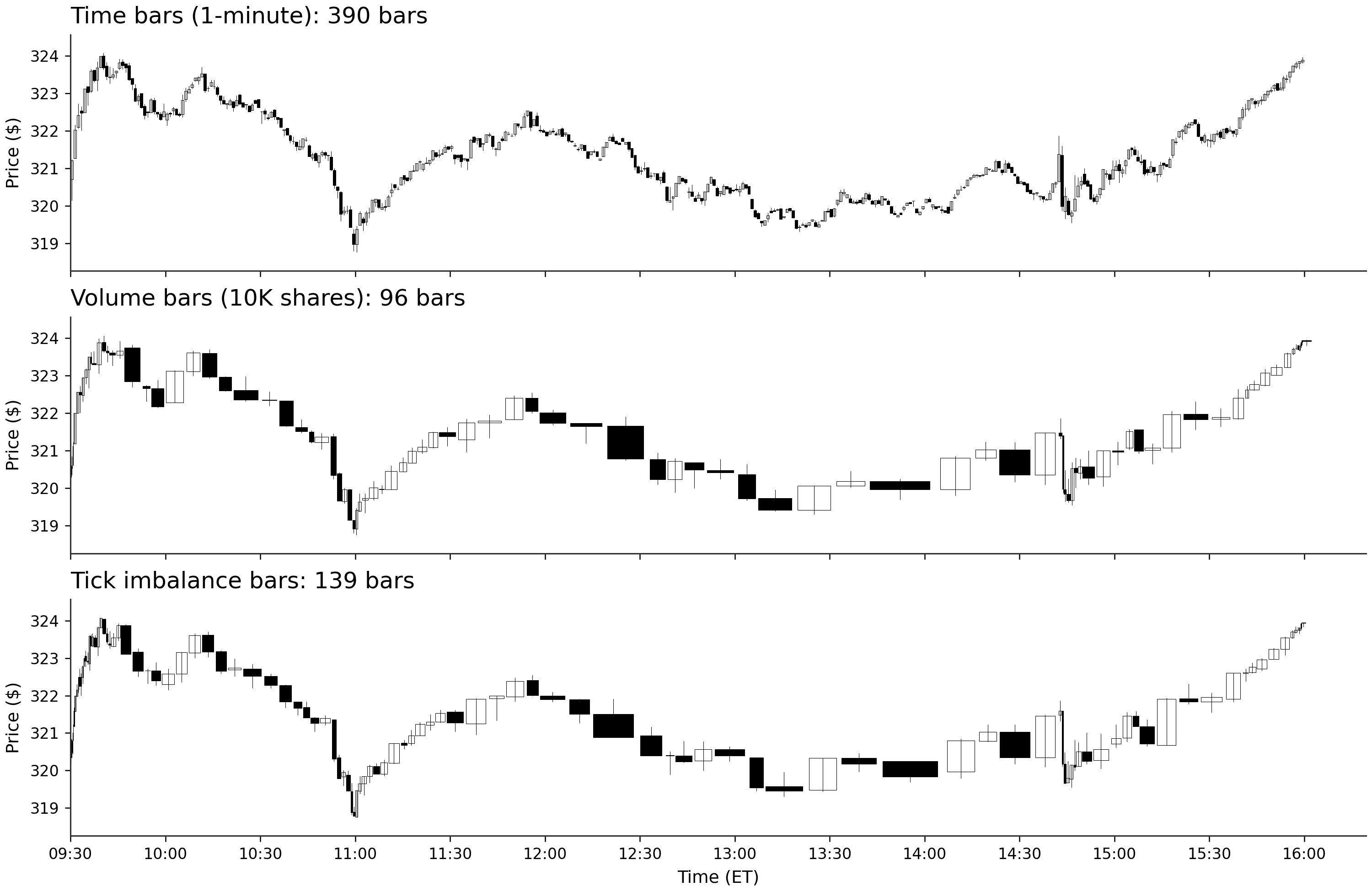
A Chapter 3 notebook turns the same AAPL trading day into one-minute bars, 10,000-share volume bars, and tick imbalance bars. The choice of sampling clock changes the observations a model receives before feature engineering begins.

Chapter 4 turns point-in-time correctness into implementation work. It covers SEC EDGAR and XBRL data, Form 4 insider transactions, 13F holdings, entity resolution, macro release alignment, CFTC futures positioning, on-chain fundamentals, prediction markets, and the extraction of filing text for later NLP work. Financial information must be aligned with the time it became available, as well as the fiscal period or event it describes.

Chapter 5 handles synthetic data with a practical standard: fidelity, utility, and privacy. Generated histories are useful when they stress robustness claims and privacy constraints; extra sample count alone cannot make a backtest more convincing.

From dataset to case study

The third-edition case studies begin with a market, a universe, a decision schedule, and a data definition. The case-study table in the main README is already public; the detailed case-study notebooks will be included in later release batches.

The futures path shows the point. A CME futures example starts with contracts, sessions, UTC timestamps, roll rules, continuous-series construction, and positioning data that arrives on its own schedule. A term-structure signal built on that data depends on each of those choices before any model sees a feature matrix.

The firm-characteristics case has a different failure mode. A monthly cross-sectional result only means something if the accounting data is lagged and aligned to a point-in-time before labels and features are built. The README lists the remaining nine case studies, including the distinct S&P 500 equity-plus-options and options-only tracks.

That is why the data release comes before the model chapters. Later chapters can ask whether a model improves a score. This release sets up the prior check: whether the score was computed on a dataset whose timing, universe, costs, and availability rules would have held up against the actual research problem.

How to inspect the release

A narrow first pass works better than browsing every notebook.

Start with data/README.md. It explains the dataset catalog, access categories, loader names, storage tiers, and the quick-start commands. The repo expects the data path in a root .env file:

# In the repository root .env file
ML4T_DATA_PATH=/path/to/your/data

# Then download free datasets
uv run python data/download_all.py --free-only

Then pick one path.

If you want the lightest local setup, start with ETFs, factors, and crypto. The minimum tier is about 70 MB. Adding macro and FX data still leaves the standard tier around 75 MB, assuming the free API keys are configured. Adding the broad US-equities dataset takes the footprint to roughly 740 MB. Adding CME futures brings it to roughly 825 MB. The full setup, including the larger microstructure and reduced licensed packages, is closer to 7 GB.

That separation matters because a reproducible notebook is only reproducible within the data rights and access assumptions it declares.

A practical first pass is:

• open the data/ README;

• run one free dataset download;

• open the matching chapter notebook;

• inspect the loader output and canonical timestamp/entity columns;

• trace that dataset into the case-study table in the main README;

• then move to the Chapter 6 feasibility notebook when that batch lands.

The next ML4T Insights issues will follow the same sequence: data first, then strategy definition, labels, features, model comparison, backtesting, costs, risk, and deployment.

For the walkthrough

The June 24 Lightning Lesson starts from this data contract: choose a market, define the decision problem, build a first baseline, diagnose what failed, and make the next iteration measurable without quietly reusing the holdout.

The July 6 cohort uses the same case-study structure as the book and repo, with sequencing, feedback, and live review.

The repo gives readers the artifacts. The course adds the working cadence: turn the artifacts into a baseline, read what the baseline says, and decide what deserves the next experiment.

You can watch or star the repo to follow the staged release. The lesson is a short live walkthrough of why the release starts with the data contract before moving to models.