More than 27 chapters

How the five libraries, 112 primers, and 56 agent skills complement the 27 chapters.

The third edition of Machine Learning for Trading ships with 27 chapters (and 400+ notebooks). It also ships with five open-source Python libraries, 112 primer articles, and 56 agent skills across nine categories. Issue 1 promised to unpack what the companion material does that the chapters alone cannot. This issue is part of that unpacking — two of the libraries in detail, plus a tour of the primer set. Skills and the agent layer that consumes them get their own treatment in forthcoming issues.

Five libraries, one workflow

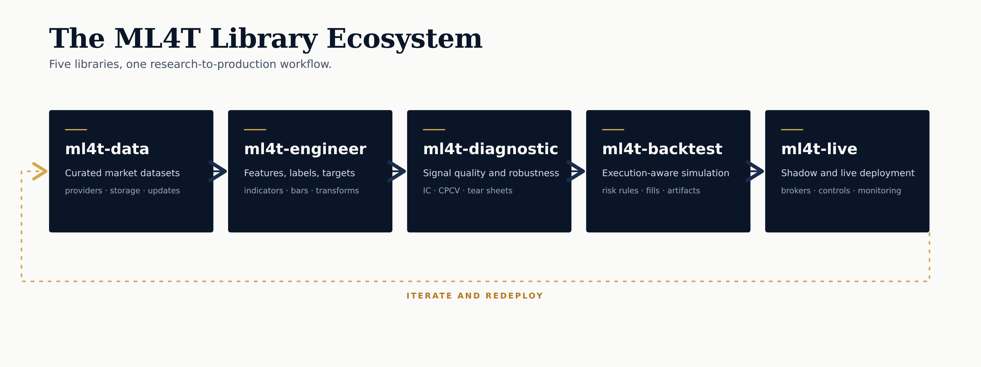
The five libraries trace the research-to-production path the book teaches: data acquisition, feature engineering, signal validation, strategy simulation and evaluation, and live deployment. Each library is finance-native — APIs, semantics, and data contracts tailored to the domain rather than borrowed from a generic ML stack. The chapters establish the methods. The library, its tests, and its validation harness ensure the methods are implemented correctly at scale.

This issue goes deeper into two areas: data management and the backtest-to-live pair.

ml4t-data: twenty providers, one interface

Most ML-for-trading projects start by writing the same data layer. Ten different vendor SDKs with ten different schemas, ad-hoc CSVs that drift out of date, and a notebook full of one-off fetches that may or may not reproduce. ml4t-data provides the data layer that the project should not have to write.

A single DataManager unifies 20+ provider adapters behind one interface — the same fetch, load, and update calls regardless of source. Coverage spans 850,000 FRED economic series, 70+ global exchanges via Finnhub, 10,000+ cryptocurrencies via CoinGecko, prediction-market history from Kalshi and Polymarket, academic factor data (Fama-French, AQR), and Databento-backed futures for CME and ICE. Data is stored locally in Hive-partitioned Parquet with metadata tracking and is queryable directly with DuckDB or Polars. CLI commands handle incremental updates, gap detection, and validation against OHLC invariants and anomaly detectors.

The two modules where lookahead bias is most likely to enter quietly get dedicated treatment. The futures module builds continuous contracts with configurable roll logic for CME and ICE products. The COT (Commitment of Traders) module joins weekly CFTC positioning data to OHLCV under explicit point-in-time semantics — the join key is the release date, not the date the positions describe — so the model never sees a Tuesday’s positions before the Friday they were published.

ml4t-backtest → ml4t-live: the same strategy, twice

The hardest move in the workflow is the move from a backtested strategy to a live one. The two environments share almost nothing by default — different data feeds, different fill semantics, different failure modes — and the bugs that survive the transition are the ones that erase paper-PnL the fastest. The backtest and live libraries are designed as a single system that cleanly crosses that boundary.

ml4t-backtest is the simulation engine, and its headline claim is cross-framework parity. Behavioral profiles for Zipline, Backtrader, VectorBT, and LEAN set dozens of knobs to match each target framework exactly so that you can either reproduce the backtester you know, or the behavior of the broker you use. Validated on 250 assets over 20 years, the Zipline profile reproduces 226,723 trades with zero gap and a $10.30 value discrepancy on the final portfolio (0.0014%), running 8× faster than the reference. The point of the parity work is to establish that the engine does what the standard implementations do, so the strategy author can stop worrying about the engine.

ml4t-live takes the same SignalStrategy class, unmodified, into production. SafeBroker enforces 16 risk parameters — position limits, order limits, daily-loss caps, fat-finger rejection at ±5% from market, asset whitelisting. Shadow mode runs the strategy logic on live data without placing real orders, closing the gap between a passing backtest and a safe live deployment. The kill switch persists atomic JSON state, so a mid-run crash does not leave orphaned positions. The design constraint is zero-rewrite migration: the code that passed the backtest is the code that runs the broker.

112 primers: a menu of choice

The second edition carried its own prerequisites. Chapters had to stop and introduce hypothesis testing, linear regression, and basic time-series mechanics. That crowded out pages for the trading applications the book was actually about. The third edition moves that material into primers and gives the chapters back to trading.

The result is a menu for you to pick and choose from along two axes:

1. Level of preparation: 20 foundational primers, 66 intermediate, 26 advanced.

2. Topic: 24 primers are cross-chapter, the other 88 provide background on or further expand on individual chapters: Ch 9 on model-based features has 11 primers, Ch 17 on portfolio construction has 8, Ch 14 on latent factors has 7.

264 unique research citations back the set. A few primers to show the range:

• “Volatility: Realized, Implied, and Why It Clusters” (Cross-chapter, foundational). Three distinct volatility objects — realized, implied, and conditional — and why they are not interchangeable. Square-root annualization explained. Volatility clustering as a potential regime marker, not an artifact of noisy estimation.

  

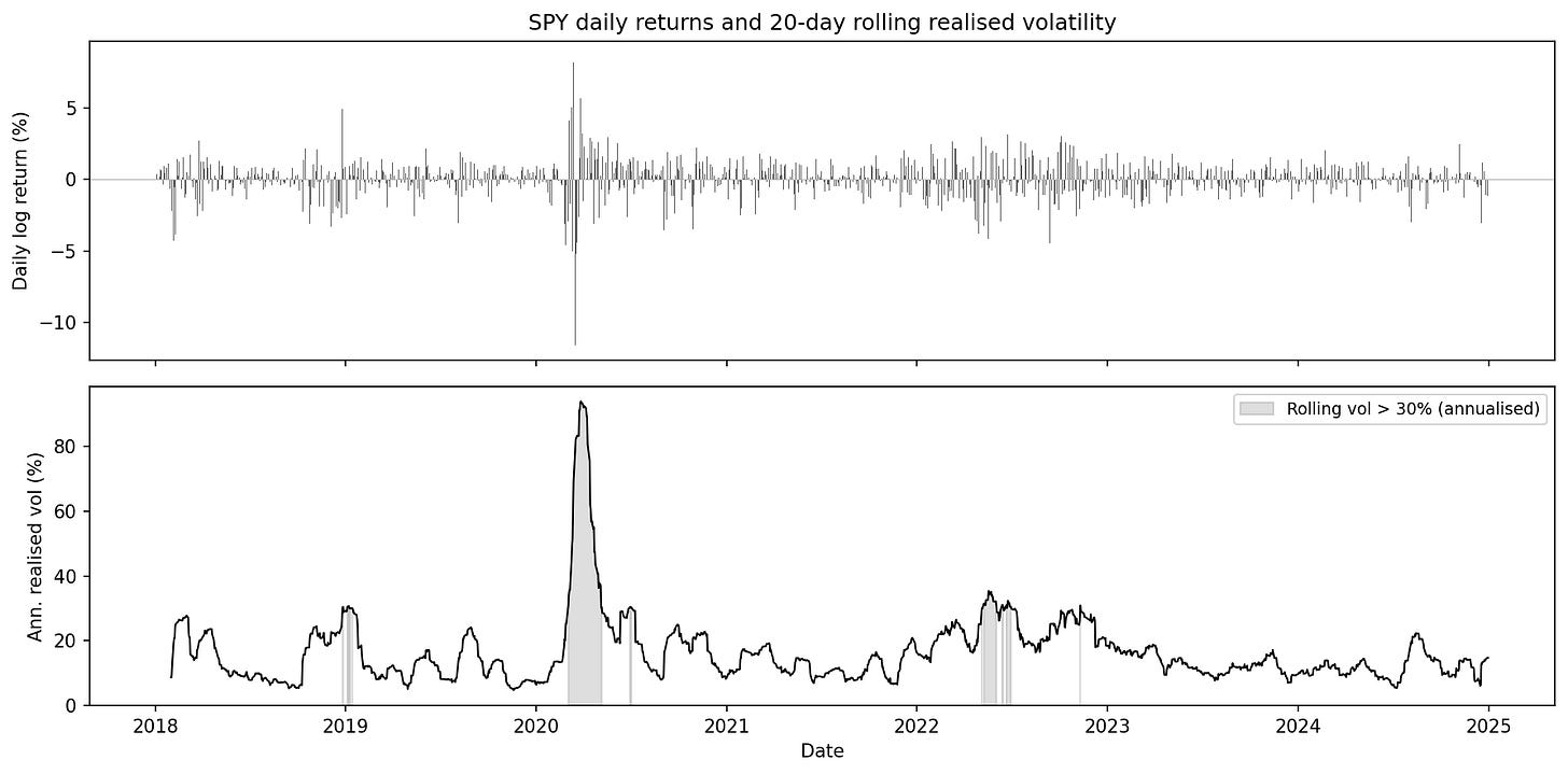
  SPY daily log returns and 20-day rolling annualized realized volatility, 2018–2024. Long calm stretches near 10–15% punctuated by short clusters — late 2018, the COVID spike to ~94%, the 2022 sell-off, and the 2023 banking episodes. Roughly 5% of days exceed 30% annualised volatility. From the primer “Volatility: Realized, Implied, and Why It Clusters”.

• “Random Matrix Theory for PCA in Finance” (Ch 14, advanced). The Marchenko–Pastur law provides a null benchmark for the eigenvalue distribution of a sample covariance or correlation matrix in the absence of structure. In finance, eigenvalues that exceed the upper edge of the Marchenko–Pastur bulk (the range of eigenvalues that finite-sample estimation noise alone can generate) are often interpreted as candidate signal components, while eigenvalues inside the bulk are treated as noise-dominated. This gives a practical, though assumption-dependent, way to decide how many principal components to retain and motivates covariance cleaning and eigenvalue shrinkage methods.

• “Temporal-Difference Learning and Bellman Equations” (Ch 21, intermediate). The foundation for value-based RL methods used in applications such as execution and hedging includes the Bellman equations, value iteration, TD(0), the bias–variance trade-off relative to Monte Carlo estimation, and the transition from tabular control methods such as Q-learning and SARSA to neural variants such as DQN and Double DQN.

What’s next

Friday’s issue opens the Agent Lab — our implementation of the multi-agent research pipeline based on Bridgewater’s AIA Forecaster that Chapter 24 teaches — running daily on live questions from Kalshi and Polymarket. The 56 agent skills and the agent layer that orchestrates the full research-to-production workflow will be included in a later issue.