How ML4T uses case studies to test strategies across markets

Nine case studies across seven asset classes, run under one research protocol.

The third edition of Machine Learning for Trading carries nine case studies: ETFs, crypto perpetuals, NASDAQ-100 microstructure, S&P 500 equity and option analytics, US firm characteristics, FX pairs, CME futures, direct S&P 500 options, and a broad US equities panel.

That list matters because the studies are not decorative applications at the end of the book. They show how the same research process performs across different datasets and in very different markets and trading environments, and each includes around 20 notebooks from data sourcing to detailed performance analysis.

They cover different asset classes, frequencies, breadths, cost regimes, and execution problems. Some are monthly. Some are daily. One is intraday. Some are long-only ranking problems. Some are long-short cross-sectional problems. One is a delta-hedged options strategy.

Model choice rarely decides whether a strategy survives. Label design, cost regime, data construction, breadth, position sizing, and search discipline usually decide it.

That is what the case studies are built to show.

That comparison space is intentionally wide. A monthly ETF rotation process, an 8-hour crypto funding trade, a 15-minute NASDAQ-100 signal, a weekly futures ranking problem, and a delta-hedged options strategy do not put pressure on the same parts of the workflow. That is why the set is useful: each market makes a different failure mode visible.

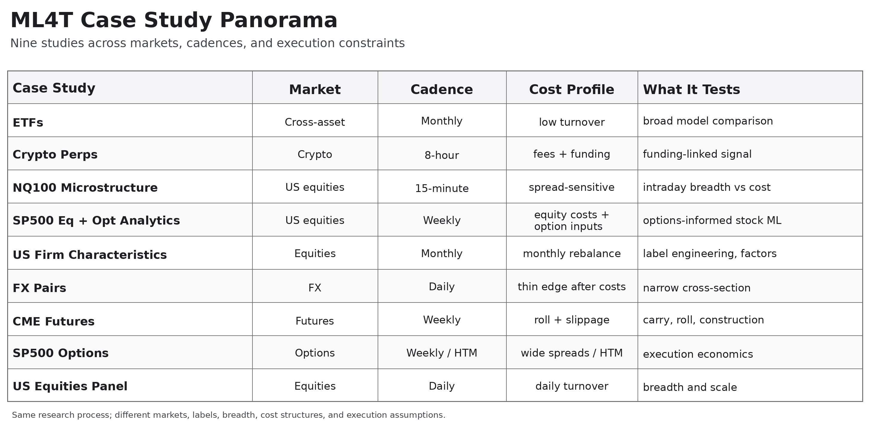
Figure 1. The point of the set is not just breadth. It is that the same research process is exposed to very different markets, cadences, and execution constraints.

What becomes comparable across nine very different markets

Because the case studies are built on the same discipline, they make more than headline Sharpe ratios comparable. A 21-day ETF label, an 8-hour crypto label, a 5-day futures label, a 15-minute intraday equity label, and a return-to-expiry options label are not interchangeable prediction problems. They encode different holding periods, execution assumptions, and cost burdens.

The same goes for features and models. Some studies rely on traditional financial features such as momentum, carry, volatility, and the term structure. Others add model-based features such as HMM regimes, GARCH volatility, or forecast model outputs. The model set is also deliberately broad: linear baselines, gradient boosting, tabular deep learning, sequence models, latent-factor models, and, where the setup supports it, causal estimators.

Just as important, the book forces the post-prediction steps into view. Signals are converted into positions, run through explicit backtests, stress-tested under costs, modified by allocators and risk overlays, and then evaluated on a holdout set. Feature ICs are measured with heteroscedasticity- and autocorrelation-corrected standard errors. Screening uses false-discovery control. Backtests are read with probabilistic and deflated Sharpe analysis, bootstrap intervals, and search-accounting adjustments. The point is not just to report a number, but to say what that number does and does not justify.

That stack is why the case studies read as research rather than as examples.

What changes once the workflow meets real markets

In the firm-characteristics study, label treatment materially changes the result. The raw 1-month return label leaves the linear baseline at an IC of about -0.005, with a HAC interval that straddles zero. On the winsorized label, the same linear family moves to about +0.023 and clears zero on a thin margin. GBM is strong in both cases, around +0.080, which is the point: the large change came from label treatment, not from swapping ridge for a more expressive architecture.

In crypto perpetuals, the problem is different. On the primary 8-hr forward return regression label, only one family leader is clearly credible: NLinear at +0.0293 daily IC with a HAC 95% interval of [+0.0168, +0.0419]. GBM, linear, and TabM all straddle zero on that same primary label. But directional reframings recover the signal for other families. That is not a “deep learning wins” story. It is a label-and-market-structure story in a small sample with only 19 instruments and two folds.

In ETFs, the comparison is broad enough to separate prediction quality from strategy quality. The study compares all major model families across a large, liquid cross-asset panel. The editorial point here is not to crown a universal winner. It is to show that the family leader on validation IC need not be the leader once the signal is turned into a strategy. The prediction problem and the portfolio problem are related but not the same.

In the NASDAQ-100 microstructure, the signal can be statistically real yet economically fragile. The current rank-1 prediction has a daily IC of around +0.0054, with a HAC interval of [+0.0022, +0.0086], indicating positive directional alignment. But the holdout strategy Sharpe still flips negative, around -1.69, and the strategy trails the equal-weight holdout benchmark. That is a clean example of why “detected signal” and “deployable strategy” are not synonyms at intraday cadence.

S&P 500 equity-plus-options analytics make a different point: options can be a useful source of information for stock prediction, but credible validation results still do not settle the execution and holdout questions.

And in direct S&P 500 options, the cost problem becomes the case study. The workflow uses a dedicated hold-to-maturity cost cascade because standard basis point grids are the wrong abstraction for the instrument. Even there, the strategy analysis says no statistically resolved edge has been earned yet. That is a useful result. It shows what it looks like when the instrument pushes back hard enough that careful modeling is still not enough.

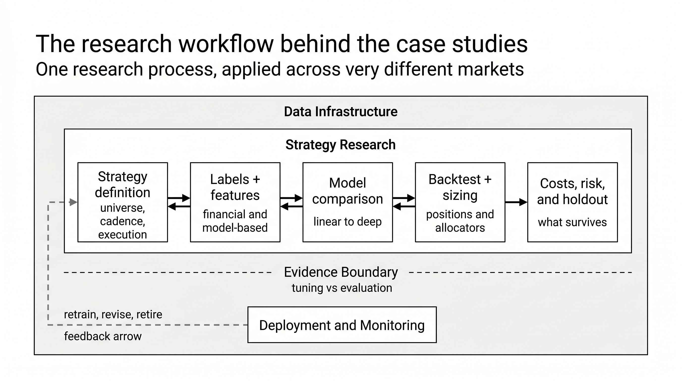
Figure 2. The same research stack repeats across all nine studies. That is what makes the differences interpretable rather than anecdotal.

Why the case studies matter

This is the real reason to read that part of the book closely.

The case studies do not just show that ML can be applied to many markets. They show how differently the same research stack behaves when the market changes.

Sometimes label engineering matters more than architecture. Sometimes costs decide the result. Sometimes breadth rescues a weak signal. Sometimes the prediction is credible, but the strategy is not. Sometimes the right conclusion is not to deploy, but to narrow the claim, change the horizon, or stop.

Because the trade definition, label design, model comparison, backtest, cost accounting, and holdout discipline are kept explicit, you can ask better questions when a strategy fails. Was the label wrong? Was the cross-section too narrow? Was the cost regime too severe? Did the signal survive validation but die in holdout? Did the apparent edge disappear once uncertainty and search adjustments were counted?

And those questions are not asked loosely. The workflow forces them through HAC IC, false-discovery control, probabilistic and deflated Sharpe, bootstrap uncertainty, and search-accounting discipline before a result is allowed to sound stronger than it is.

That is serious empirical work. And it is much closer to how real quant research feels than a neat parade of winning backtests.

Read that way, the nine case studies are not a tour of examples. They are part of the book where the whole argument is exposed to the market and forced to earn its claims.

The ML4T library ecosystem, built to support the workflow

The software stack behind that process is documented on our website and is live on PyPI:

• ML4T Data handles multi-provider acquisition and point-in-time storage.

• ML4T Engineer builds features, labels, and alternative bars;

• ML4T Models adds finance-native latent-factor, SDF, direct-prediction, and portfolio-learning models;

• ML4T Diagnostic covers IC analysis, false-discovery control, Deflated Sharpe, Rademacher, PBO, CPCV, and tearsheets; and

• ML4T Backtest turns signals into event-driven strategy results with explicit execution, risk, and account rules.

Together, they make the case studies reproducible rather than descriptive.