

From Research to Production with Nine Case Studies
A hands-on ML4T course built on nine case studies: one research workflow from feasibility through deployment — equities, options, futures, FX, and crypto.

This summer we’re opening the first cohort of Machine Learning for Trading: From Research to Production — a hands-on course built around nine case studies, where you take one trading strategy from a first feasibility check all the way through deployment. See course page and overview video for more details.
Here is the kind of problem that workflow has to handle.
One of those nine case studies runs the ML4T workflow on thirty CME futures, daily, from 2011 through 2025. The model is a gradient-boosted ranker on a five-day forward return, traded as a long-short book — long the top-ranked contracts, short the bottom, inverse-volatility weighted across both sides. The label that feeds it is built on a ratio-adjusted continuous price series: back-adjusting the price level at each contract roll keeps the roll gap from registering as a price move, so it never lands in the forward returns the model trains on. Leave the series unadjusted and every roll embeds that artifact. Both decisions matter, and so does the validation around them: the result is measured on a holdout never touched during model selection, and against a long-only equal-weight basket of the same contracts.
Put together, they hold up. The validation Sharpe — the inverse-vol book under a 5% trailing-stop overlay — is 1.36, and on the 2024–2025 holdout it comes in at 1.11 — close enough that the profile carries, though the window is short enough that the gap between the two is not statistically resolved. The robust part is the signal itself: a daily information coefficient near 0.03 that clears the 5% significance threshold on both windows (on autocorrelation-robust standard errors, since the five-day labels overlap), and a result that survives the cost model — a Sharpe near 1.0 net of a tick-implied trading cost of about 10 basis points of notional per leg (modeled, not realized fills), against a breakeven near 30 basis points per leg, a roughly threefold cushion. It sits above the long-only basket too (about 0.6 in validation, 0.8 on the holdout), though a long-short book against a long-only directional basket is a floor rather than a risk-matched comparison. In this market the data construction shapes the result just as much as the model family does: get the roll handling wrong and even the cleanest model trains on a price path you could never have held. The case works because the data, the model, the cost model, and the holdout each carry their weight, and the workflow is built to show which stage carries how much.
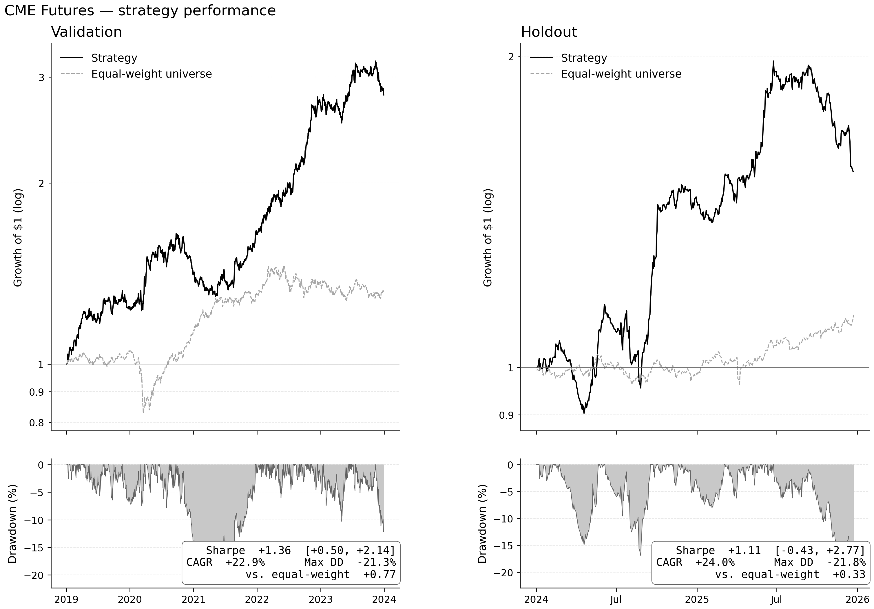
Validation (left) and a holdout the model never saw (right), each against a long-only equal-weight basket of the same thirty contracts. Validation Sharpe 1.36; holdout 1.11 — the profile carries across the split.
None of those decisions is glamorous on its own: most of a strategy’s fate is settled in the handoffs between stages, not in the choice of model. We ran this loop nine times, and the new cohort is built so you run it too: you walk away with the workflow and one case you took all the way through yourself.
That workflow is the same on every case: a feasibility check, labels and features, a ladder of models, backtesting, portfolio construction, cost and risk analysis, an out-of-sample holdout, the deployment path, and the monitoring after. Running it nine times is what makes the handoffs visible: the decision that carries each case moves from one market to the next, so you learn the pattern instead of one example. Every run is logged, and you keep the notebooks, the run registry, and the deployment scaffold.
The comparative lab
The pipeline is fixed; what it has to handle changes with the market. ETFs anchor the set as a shared reference — daily frequency, an inspectable universe, a cost model you can reason about, an allocator you can deploy — and the other eight show how the same workflow adapts when the market does.
The two S&P rows describe different problems on the same underlying: one uses options data as side information to forecast equities; the other trades the options directly — the same instrument posed as two different trading problems. Each setting shows where an edge comes from, and how much of it survives once costs and capacity are real.
What the workflow forces you to confront
A working pipeline, stage by stage, in the same numbered sequence on every case — one notebook per stage, mapped to the chapter that teaches it:
Feasibility — confirm the universe and its cost structure can support a strategy before you model anything; the straddle case is a feasibility problem before it is a modeling one.
Labels and features — forward returns at the horizon you actually trade, walk-forward splits, and features from momentum and carry to model-based ones: walk-forward GARCH, HMM regimes, particle-filtered stochastic volatility.
A model ladder — linear baselines, Optuna-tuned gradient boosting, neural tabular and sequence models, latent-factor methods, and double machine learning for the causal question.
Strategy construction — backtest, covariance cleaning with random-matrix methods (following Paleologo’s treatment), an instrument-appropriate cost model, and risk overlays.
Validation — an out-of-sample holdout scored with deflated performance measures and multiple-testing corrections.
Production — a deployment loop, then drift monitoring once it is running.
The work that decides the outcome lives in the handoffs between these stages, and one principle keeps reappearing: use only data you would have known at decision time. In the CME opener it was building the label on a roll-adjusted series, so the model never learns from a continuation no one could have traded. In NASDAQ microstructure it is bar-close timestamps — whether an order-book feature was observable when the 15-minute bar closed. In the firm-characteristics panel it is reporting lags and restatements, aligning each fundamental field to the date it was actually known. Different markets, same decision, and it separates a tradable result from a notebook artifact — which you only learn by working the case.
The record, and the right to deploy
Model work is where people expect the course to get technical. It does, and the discipline that makes it pay off is being able to prove, six weeks later, exactly what you ran.
Every training run, prediction set, causal estimate, and backtest is written to a run log: a SQLite registry where each entry is content-addressed by a hash of its full configuration, with its artifacts and results recorded against that hash. A hyperparameter sweep becomes an auditable archive you can query rather than a folder of guesses. That is what makes a model comparison honest: the synthesis step reads the registry to recover how many configurations you effectively tried, then scores each candidate against that count — deflated and probabilistic Sharpe ratios, multiple-testing corrections, the probability of backtest overfitting, and a block-bootstrap comparison against an equal-weight benchmark. (The deflated-Sharpe and overfitting measures are López de Prado’s.) Your best result is judged against the number of attempts it took to find it, and then it meets an out-of-sample holdout it has never touched.
When validation and the holdout agree, you have evidence to carry the strategy forward: paper trading, limited deployment, or further monitoring. The firm-characteristics case is the cleanest version of that agreement: a monthly cross-sectional ranker over roughly 2,500 US stocks whose validation Sharpe of 2.75 carries to 1.77 on a holdout the model never saw, with its drawdown profile holding intact alongside the Sharpe — the cleanest such transfer of the nine. When validation and the holdout disagree instead, the course teaches you to read why — whether the prediction degraded, the portfolio translation lost it, or the regime changed. Where a causal question is well defined, a double-ML treatment-effect estimate with a refutation test asks whether the relationship survives a different specification — a separate question from whether the strategy is tradable after costs. That diagnostic ability is what lets you tell the strategies worth more of your time from the ones that are not.
Through deployment, and after
A research result is not the finish line. The deployment chapters run the strategy as a live loop: a unified framework that shares feature and signal code between research and live paths so they cannot silently diverge, a verification step that checks that parity, an order state machine, broker integrations for paper and live trading, and runtime safety controls. In the cohort, deployment means standing up that loop and its controls; committing capital stays your decision. The monitoring chapters cover what happens once it is running: drift detection on features and predictions, circuit breakers, safe model rollout, and a feature store so the live system reads the same features it was trained on. This is running code — the ETF, crypto-funding, and FX cases each have a working deployment loop.
In the cohort
You take one case study — or your own data, if it fits the scope — and run the arc end to end: a clean baseline, a hypothesis about its binding constraint, two or three targeted cycles, each change tested against an out-of-sample holdout under the same protocol. Some changes hold up; some do not, and the cohort is built around learning to tell them apart. What you produce is a research package and the verdict it earns — advance, revise, or retire — scored against a rubric you see on day one.
Coding agents work inside that same protocol. The third edition ships an ml4t-skills companion — 61 skills mapping specific failure modes (leakage, lookahead, purging, cost models, capacity, deployment) to checks an agent runs in your editor, browsable now with a free account at https://www.ml4trading.io/skills/. Agents speed up loaders, tests, and ablations; the skills keep that speed inside the research protocol so the code stays correct as it gets faster.
Logistics
The first cohort starts Monday, July 6, 2026, and the first live session is Thursday, July 9, at 4 PM UTC. The format is eight weekly 90-minute cohort sessions on Thursdays — twelve hours of live class — plus four biweekly 60-minute office-hours sessions, and a final 30-minute one-on-one discussion with me about your project. Every session is recorded and posted within a day, so nothing is lost if you miss a live hour. Between sessions, support runs through a dedicated Discord server, so questions on your case do not have to wait for the next session.
The book publishes in the coming weeks: chapters one through ten are already public, with the case-study code rolling out after, and cohort members get everything they need from day one. Several cases run on free, open data; the intraday microstructure work uses institutional AlgoSeek data, provided to every cohort member along with the rest of the course material.
The best fit is a reader who can already build a complete strategy and wants to get better at the research itself. By the end you have a complete case-study research package — the workflow, the diagnosis and experiments behind your result, your out-of-sample evidence, and the means to repeat all of it on your own data.
See course page and overview video for more details.