


Most machine learning workflows for trading stop before the trade.
A model estimates returns, ranks assets, or emits a signal. A risk model estimates covariance or volatility. An allocator turns those objects into weights. A backtest then decides whether the chain produced a portfolio worth trading.
That separation is valuable because it makes errors easier to diagnose. If the signal has no information coefficient, the allocator is not the first suspect. If the signal has a positive IC but the strategy loses money, the next checks are sizing, turnover, costs, concentration, exposure, and timing.
End-to-end portfolio learning changes the object being learned. The network maps market features directly to positions and trains on a portfolio-level objective, usually a differentiable Sharpe-style loss computed after volatility scaling and turnover costs. The appeal is alignment: the gradient flows through a portfolio return stream closer to the object used in evaluation, rather than stopping at one-step forecast error. The risk is that forecasting, sizing, turnover, and exposure control become entangled in one loss surface.
The practical rule is narrow: use end-to-end allocators when the objective cannot be cleanly decomposed into forecasts plus an optimizer, and evaluate them as full trading systems rather than allocator modules. Objective alignment is not evidence. It is a reason to run stricter evidence checks.
Chapter 17 of Machine Learning for Trading uses this tension to place learned allocators inside a broader portfolio-construction workflow. The chapter does not argue that neural allocators replace classical allocation. It asks a narrower question: when is it useful to train the allocation decision itself?
Three recent lines of work make the progression visible. The first shows that portfolio weights can be trained directly through a Sharpe-style objective. The second asks which sequence architectures survive under a common volatility-targeted portfolio loss. The third adds structure: cost-aware training, cross-market filtration discipline, graph-constrained attention, and a robust regime objective.
Chapter 17’s ETF examples use those papers to ask a practical question: what has to be checked when the model owns the path from features to weights?
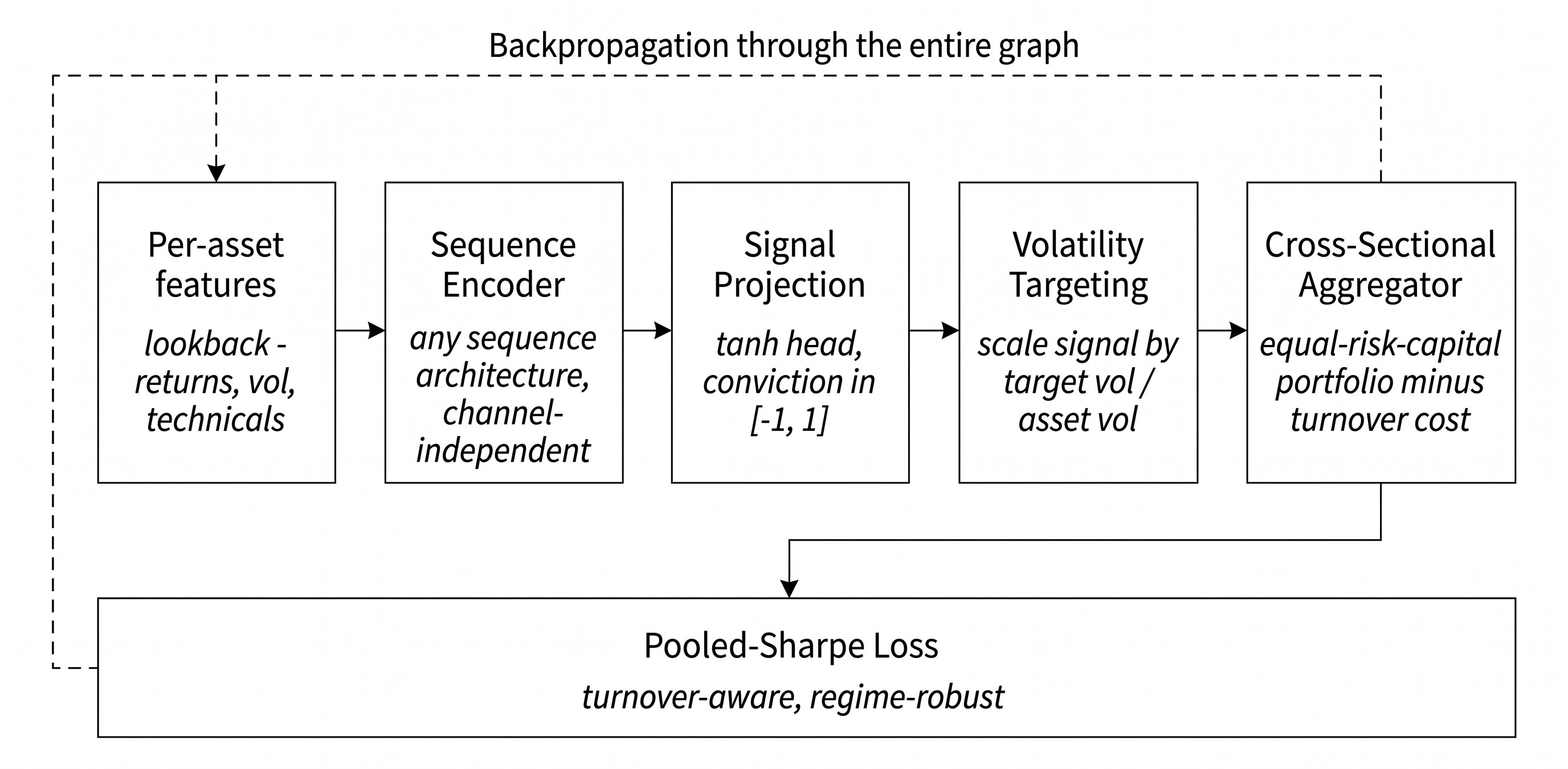
Figure 1. The end-to-end portfolio-learning pipeline in Chapter 17. Per-asset features pass through a shared sequence encoder, a bounded signal head, a volatility-targeted position layer, and a portfolio-return aggregation step. The loss is a risk-adjusted statistic of realized portfolio returns, so gradients flow through the allocation decision rather than stopping at a forecast.
What changes when the model learns weights
Chapter 17 starts with a portfolio-construction term sheet: objective, inputs, constraints, rebalancing protocol, cost treatment, and evaluation plan. That framing matters because allocation is otherwise easy to turn into an unlogged search layer once model selection is complete.
The early sections cover the standard allocator workflow. Expected returns may come from a model. Covariance may come from a shrinkage estimator, a factor model, or a realized window. Constraints and turnover penalties shape the final weight vector. Evaluation then asks whether the allocation improved the portfolio relative to a benchmark allocator, using the same signal and backtesting protocol.
The learned allocators in Section 17.8 are different. They do not consume the same forecast stream as the allocator comparisons earlier in the chapter. They learn from raw or engineered price features and output positions directly. A head-to-head table is still useful, but it compares systems rather than allocators fed identical predictions.
That makes learned allocators a separate evidence track. They are not allocator modules fed identical forecasts; they are full trading systems. They must still pass simple heuristics, but the comparison must include leakage checks, costs, turnover, drawdown, regime slices, seed variation, and component ablations. A single test Sharpe is not enough evidence when the model owns the entire path from features to weights.
The tables below should be read as experiment-specific evidence, not as a single consolidated leaderboard across different data masks, model protocols, and portfolio-return calculations.
The common computation graph
The three implementations share a recognizable core graph, although their constraints, cost treatment, and details of the robust objective differ.
For each asset and decision time, the model receives a fixed-length lookback window. A sequence encoder processes the window and produces a hidden state. A small head projects the hidden state into a signal. A position layer converts the signal into a tradeable weight, usually after volatility scaling. The portfolio-return layer combines those positions with next-period realized returns and subtracts turnover costs. The training loss is computed on the resulting portfolio-return stream.
The base loss is usually a negative annualized Sharpe-style objective computed over the portfolio return stream. It rewards average portfolio return relative to portfolio volatility rather than one-step forecast accuracy. Later versions add cost terms and robust subperiod penalties. The notation is schematic: the papers and examples differ in output constraints, volatility scaling, transaction-cost treatment, and robust-window construction. Figure 2 puts the objective where it belongs in the workflow: weights, returns, masks, costs, and previous positions first form a net return stream; the loss then rewards pooled Sharpe while adding pressure on weak subperiods.
The pooled Sharpe term asks whether net portfolio returns compensate for realized volatility after sizing and costs. The SoftMin term is a smoothed worst-window Sharpe ratio; maximizing it rewards policies whose weak windows improve rather than those that rely on a few favorable windows.
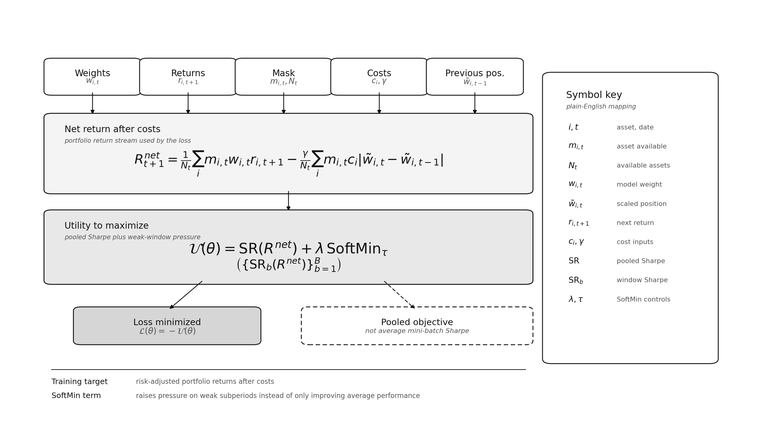
Figure 2. The portfolio objective is built from current weights, next-period returns, availability masks, previous positions, and cost inputs. The formula is shown as a schematic rather than an implementation identity; the symbol key defines the notation used in the image.
Two details are easy to understate.
First, the pooled Sharpe is not a separable loss. Its gradient depends on the mean and variance of the return stream. If a training loop computes Sharpe in small mini-batches and averages the resulting gradients, it optimizes the average mini-batch Sharpe, not the pooled Sharpe across the full panel. Those objectives can prefer different policies because the denominator is computed on different return distributions.
DeePM treats this as an implementation issue, not a footnote. The paper introduces an exact two-pass microbatching procedure for large effective batches:
First, accumulate sufficient statistics for the full logical batch, then replay the forward pass with the corrected normalization so the gradient matches the pooled objective.
Second, cost-aware training differs from post hoc cost reporting. If turnover costs are charged only after training, the model can learn a policy that works on gross returns and fails when traded. When costs are within the return stream being optimized, the model encounters implementation friction during training.
Direct Sharpe training is only the start
Zhang, Zohren, and Roberts (2020) provide the clean starting point. The paper bypasses the expected-return forecast and trains a neural network to output long-only portfolio weights directly. A softmax layer keeps weights positive and ensures they sum to 1. The objective is portfolio Sharpe computed from realized portfolio returns, and gradient ascent updates the model parameters.
The paper deliberately keeps the architecture simple: a single-layer LSTM with 64 units, a 50-day lookback, close prices and daily returns as inputs, Adam optimization, and a validation split for hyperparameter control. The empirical setup uses four ETFs or index proxies: VTI, AGG, DBC, and a VIX-tracking proxy. Reported test results include volatility scaling and transaction costs. In that four-asset setting, the deep learning strategy performs well relative to the paper’s baselines and moves substantially toward bonds during the COVID-19 crash, which falls inside the paper’s test period.
The novelty lies in the objective, not in architectural complexity. The model demonstrates that portfolio weights can be learned via a differentiable, risk-adjusted objective without first estimating expected returns.
The Chapter 17 ETF example is useful precisely because it does not flatter the method. It puts the same idea into a broader 29-ETF setting, using daily prices from 2006-01-03 to 2025-12-31, a chronological 60/20/20 train/validation/test split, 63-day sequences, and a long-only softmax LSTM trained against a differentiable Sharpe objective.
The result is a useful negative control:
The learned LSTM reduces volatility and drawdown, but the return side does not compensate. Equal weight and inverse volatility are not straw-man baselines here; they are low-turnover controls that expose whether the learned policy earns its extra complexity. The best validation Sharpe is 1.609; the test Sharpe is 0.48. Directly optimizing a portfolio loss does not remove overfitting. It moves the overfitting target from prediction error to the portfolio object itself.
This is why the baseline belongs in the issue. It prevents the argument from becoming “train the Sharpe and win.” The paper establishes the training principle. The Chapter 17 replication shows why the principle needs stronger architecture, costs, and validation discipline before it becomes competitive.
Better sequence models still have to pay costs
Saly-Kaufmann et al. (2026) ask the next question: if every model is evaluated under the same portfolio objective, which temporal architecture earns its complexity?
Their benchmark uses roughly 15 years of futures and currency data across bonds, commodities, energy, foreign exchange, and equity indices. Each model maps a lookback window to a bounded signal in [-1, 1]. A volatility-targeted position layer converts the signal to risk-scaled exposure. The paper uses pooled Sharpe as the optimization objective and reports a broad set of evaluation metrics: annualized return, Sharpe ratio, HAC statistics, hit rate, turnover, passive-relative information ratio, downside risk, seed robustness, and breakeven transaction costs.
The paper evidence is best read as an architecture ranking under a shared protocol, not as a claim that those absolute Sharpe ratios transfer to the Chapter 17 ETF examples. The benchmark uses a different universe, futures-style instruments, a 10% volatility target, seed averaging, and a different implementation stack.
Within that benchmark, the main lesson is not that one architecture universally wins, but that inductive bias matters more than raw capacity. VLSTM, a variable-selection network in front of an LSTM encoder, reports the strongest aggregate Sharpe in the main table: 2.39, with a 23.9% annualized return. The hybrid LPatchTST and TFT are close behind, at 2.32 and 2.20, respectively. xLSTM has a lower average Sharpe ratio of 1.80 but a more favorable turnover profile than the classical LSTM, which matters for implementation. iTransformer has very low turnover but weak economic performance, with a Sharpe of 0.35 in the reported benchmark.
The discussion is more important than the ranking. Recurrent or recurrent-hybrid models do well because the architecture builds in a temporal axis rather than forcing the model to infer it from noisier token structure. Variable selection helps because most financial features are weak, unstable, or regime-dependent. But the “best” architecture depends on the metric. VLSTM leads on average Sharpe; LPatchTST and VxLSTM, the variable-selection plus xLSTM hybrid, look attractive on some downside and tail-risk measures; xLSTM has a stronger cost buffer in the paper’s breakeven analysis.
The paper also checks seed sensitivity. Under a smaller experimental budget, VLSTM still reports a Sharpe near the full-budget estimate: 2.40 in the reduced-seed table versus 2.39 in the main table. That does not make the result universal, but it reduces the risk that the ordering is only a lucky initialization artifact within this benchmark.
The Chapter 17 VLSTM example applies that idea to the same ETF universe. It keeps the same 29 ETFs, the 2006-2025 price panel, the 63-day sequence length, and the chronological split as in the first ETF example. The model changes the allocator in two ways:
It adds a TFT-style gated residual network and variable-selection network before the LSTM;
It replaces the softmax long-only output with a volatility-targeted long-short position layer trained with a 5 bps cost-aware pooled-Sharpe loss.
The cost table below is an out-of-sample stress test on one trained model. The model is trained with a 5 bps one-way cost inside the loss; the table then revalues the same held-out weights at 0, 5, 10, 20, and 50 bps one-way cost per dollar of turnover. It is not retrained at each cost level.
At zero cost, VLSTM is effectively tied with equal weight. The cost profile is the result that matters:
The VLSTM variant recovers most of the gap between the softmax LSTM and the heuristic allocators at zero cost. It does not survive the 5 bps cost assumption used during training. That is a substantive result, not a caveat. Architecture can look competitive and gross, yet still fail the deployability test.
Robust portfolio learning needs structure
Wood, Roberts, and Zohren (2026) advance the same line of work. DeePM is built for systematic macro portfolios, where the model must learn from noisy non-stationary data, trade across asynchronous global markets, and survive transaction costs.
The paper identifies three design problems.
The first is the ragged filtration problem. Global markets do not close at the same time. A naive cross-sectional attention layer can inadvertently allow an earlier-closing market to see information from a later-closing one. In the paper’s implementation, Directed Delay lags cross-sectional conditioning so that cross-market representations are measured with respect to a common information set, preferring filtration discipline over maximum same-day freshness.
The second is low signal-to-noise cross-asset learning. Free attention can form economically implausible links and overfit unstable correlations. DeePM uses a macro graph prior: an ex ante economic topology that constrains or biases cross-asset attention toward admissible relationships. The paper gives examples such as intra-group cliques, risk-on links across equities and cyclical assets, and inflation-sensitive links among energy, rates, and precious metals. The graph is a structural regularizer, not a claim that the specified edges are ground-truth causality.
The third is regime fragility. A pooled Sharpe objective can be lifted by favorable windows while hiding weak periods. DeePM augments pooled Sharpe with a SoftMin penalty over subperiod Sharpe ratios. As the temperature approaches zero, the penalty approaches the worst window. At intermediate temperature, it emphasizes weak windows without collapsing onto a single episode. The paper connects this to a KL-penalized distributionally robust objective and to Entropic Value-at-Risk.
The architecture maps those problems into explicit modeling choices:
a vectorized variable-selection network with FiLM-style static conditioning, where static asset context modulates features through feature-wise affine transforms;
an LSTM temporal backbone plus temporal attention;
lagged cross-sectional attention for filtration discipline;
macro-graph attention for economic structure;
a cost-aware net-return objective;
a SoftMin-augmented robust Sharpe loss.
In the DeePM paper’s 2010-2025 macro futures test, with out-of-sample returns rescaled to a 10% annualized volatility, the full model reports a gross Sharpe ratio of 1.29 and a net Sharpe ratio of 0.93 after transaction costs. Passive equal risk reports a 0.50 net Sharpe ratio, TSMOM 0.45, and the Momentum Transformer baseline, trained with the same transaction-cost regularization, reports 0.66. The paper-level ablations matter:
Those are paper results on a 50-contract futures and FX universe, not results from the Chapter 17 ETF examples. The distinction matters.
The local ETF example then asks a narrower practical question: what happens when a DeePM-style structure is adapted to the same setting? The example uses 29 ETFs, five asset-class groups, daily prices from 2006 to 2025, an 84-day sequence length, and a chronological 60/20/20 split. It includes FiLM conditioning, variable selection, an LSTM backbone, cross-sectional attention, a small ETF macro graph prior, transaction costs, and the SoftMin objective. The key contrast is full DeePM versus a no-SoftMin ablation.
One protocol detail prevents a bad cross-table comparison. The heuristic baselines are local controls within each example, not a single shared benchmark series. The LSTM and VLSTM examples evaluate final-step returns from sliding windows; the DeePM-style example evaluates the full post-validation test-date mask and normalizes model risk weights before computing returns. The equal-weight rule is not changing; the sampling and return-alignment protocol is. Read each table within its local comparison, not as a claim that the same equal-weight series has two different Sharpe ratios.
On the test window:
The regime slice explains the source of the improvement. The split is mechanical: test days above the median 21-day annualized realized volatility of SPY are labeled “crisis,” and the remaining days are labeled “calm.” In this run, the threshold is set to 14.0%, resulting in 504 calm days and 503 crisis days.
SoftMin does not help by making calm periods better. Calm Sharpe falls slightly from 1.26 to 1.21. The improvement comes from the crisis side, where Sharpe rises from 0.57 to 1.00. In this ETF window, the robust objective improves the shape of losses and the average statistic simultaneously.
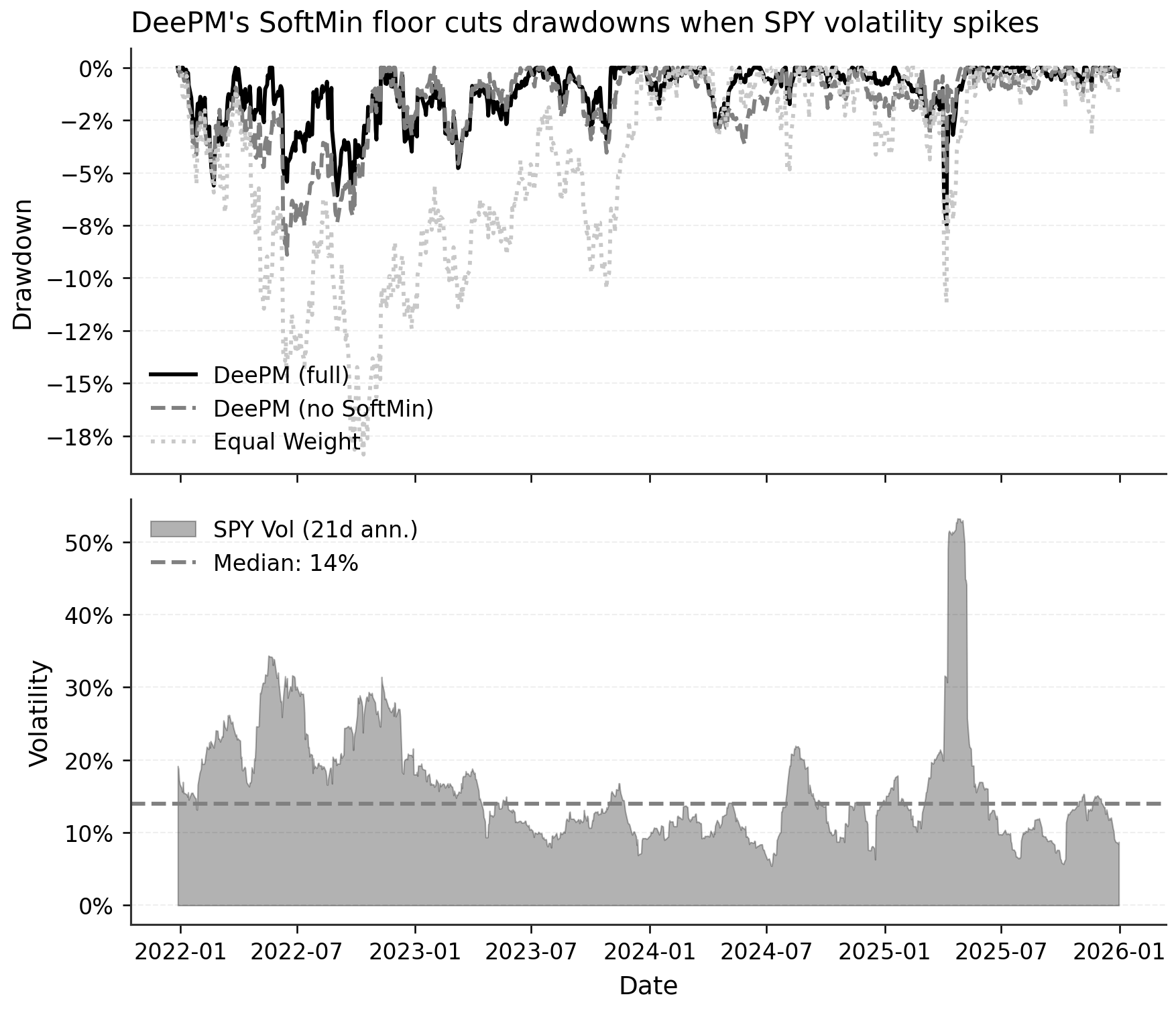
Figure 3. DeePM drawdown comparison from Chapter 17. The full SoftMin version keeps drawdowns shallower during high-volatility periods than the equal-weight and no-SoftMin ablations. The point of the figure is the path of losses, not only the full-window Sharpe ratio.
The ETF example does not isolate every DeePM component. It does not separately quantify FiLM, V-VSN, Directed Delay, macro graph, and temporal attention as the paper’s broader ablation table does. Its measured local contrast is full DeePM versus no SoftMin, with the architecture held otherwise fixed. The example also does not run a DeePM cost-stress grid, unlike the VLSTM table, so the result should not be taken as proof that the ETF DeePM policy survives arbitrary cost assumptions. The ETF Sharpe ratio should also not be read as evidence that the reduced example system is better than the paper system; the asset universe, volatility target, training protocol, ensemble design, and cost model differ.
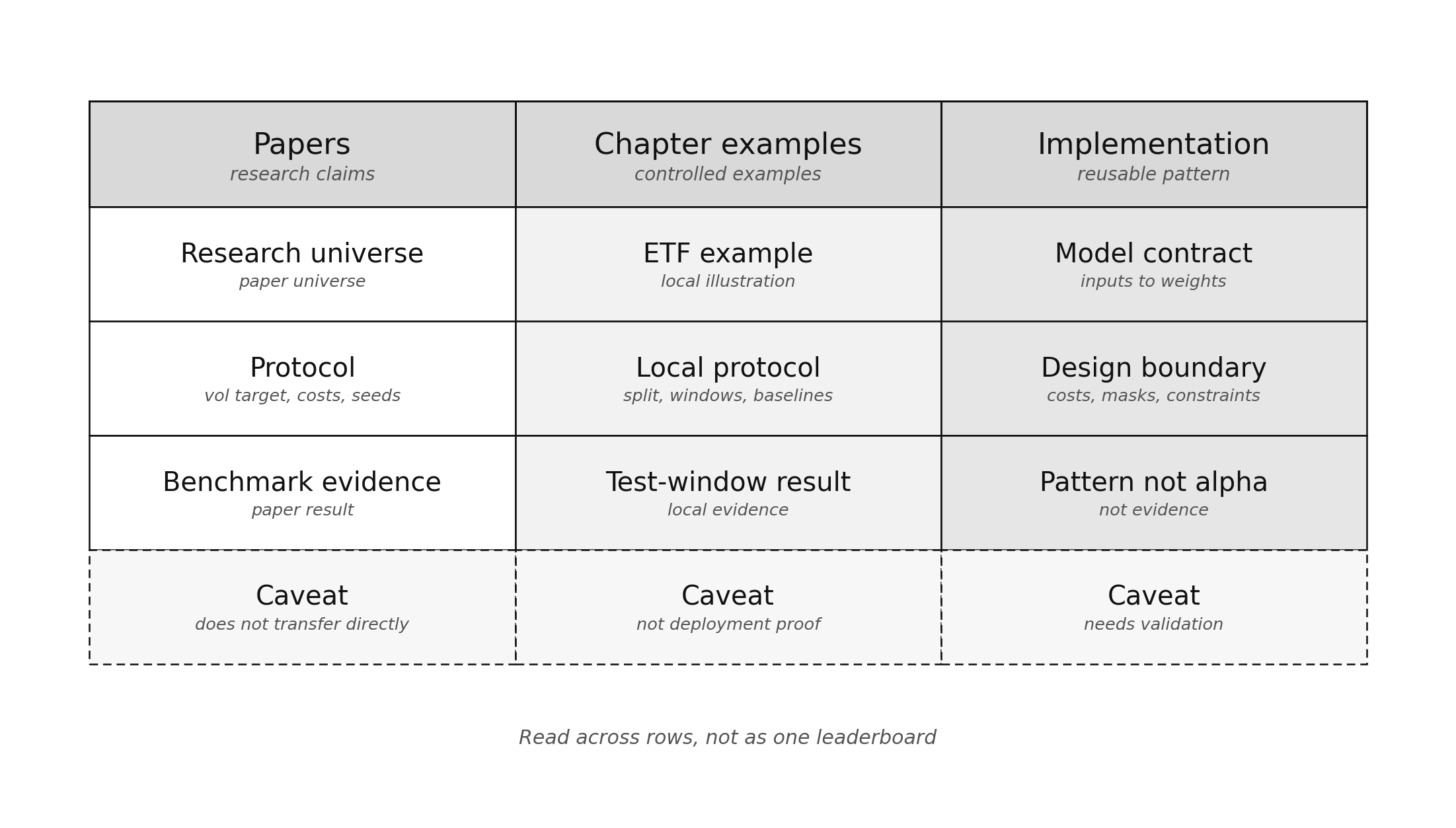
Figure 4. Papers, Chapter 17 examples, and implementation patterns answer different questions. Paper benchmarks support research claims; local ETF examples illustrate evaluation logic; implementation patterns preserve the contract, not evidence of alpha.
The implementation contract
The evidence boundary is now the main point: papers, Chapter 17 examples, and implementation patterns answer different questions.
The reusable lesson is not a list of class names. It is the contract an end-to-end allocator has to preserve: what the model needs to see, what it produces, and where downstream constraints belong.
For a learned allocator, the input contract must carry more than just features. It needs feature windows, forward returns, availability masks, volatility-scaling terms, cost inputs, previous weights, and, when used, economic graph structure. The output is not a forecast to be handed to a separate optimizer; it is a target weight vector that must still pass through exposure, leverage, turnover, and backtest checks.
Each part of that contract corresponds to a failure mode from the papers and examples:
This is the implementation boundary that matters. A DeePM-style allocator is not just a generic sequence model with a Sharpe loss. It needs a net-return layer, cost-aware turnover, pooled-objective semantics, optional graph constraints, and hooks for portfolio constraints after the model emits weights.
At the same time, packaging those mechanisms in software is not evidence of alpha. The evidence still comes from matched protocols, out-of-sample tests, cost stress, regime slices, seed checks, and ablations.
Alignment raises the burden of proof
The evidence across the Chapter 17 examples is mixed.
The softmax LSTM shows that direct Sharpe training can underperform simple heuristics. VLSTM shows that a better architecture can improve gross performance and still lose after costs. The reduced DeePM-style ETF example shows that, in this test window, a structured allocator with the SoftMin objective improves Sharpe, drawdown, and crisis-window performance relative to its local controls.
End-to-end training is not a shortcut around portfolio-construction discipline. It is a way to move more of the trading problem into the learning objective. Once that happens, the validation burden grows. The 0.98 versus 0.69 DeePM comparison is evidence from one ETF test window; it still needs seed, cost, period, and ablation checks before it can support a deployment claim.
A learned allocator should be judged by a protocol tied to the failure modes above:
Start with heuristic baselines. The softmax LSTM does not assign equal weight or inverse volatility to the ETF window.
Report gross and net performance. VLSTM’s zero-cost tie disappears at 5 bps one-way cost.
Show turnover and cost-stress curves. A cost-aware loss can still learn weights that are too expensive out-of-sample.
Slice regimes with a rule defined before looking at results. The DeePM example uses median SPY realized volatility.
Report seed sensitivity where the model class makes it material. Saly-Kaufmann’s reduced-seed check is part of the evidence, not a footnote.
Use ablations when the claim is architectural. DeePM’s paper-level result is more credible because the no-SoftMin, no-graph, and graph-only variants are visible.
This is where Chapter 17’s workflow matters. Classical allocators remain the right default when signals, risk estimates, and constraints can be diagnosed cleanly. End-to-end allocators become more compelling when the objective is hard to factor into a forecast plus an optimizer: cost-aware sizing, regime robustness, or structured cross-asset interaction.
The practical takeaway from this line of work is not that deep learning beats portfolio heuristics. It is that portfolio-objective training can align the model with the economic target, but only if the architecture, cost model, and evaluation protocol are strong enough to carry that alignment out-of-sample.
The Chapter 17 examples show the experimental progression, not trading instructions. The implementation lesson is the same throughout: sequence information in, target weights out, with costs, volatility scaling, graph structure, and robust Sharpe treated as first-class parts of the model rather than afterthoughts. Direct portfolio learning is not a replacement for portfolio construction. It is portfolio construction moved into the model, which makes the modeling problem more aligned and harder to audit.
Hi Mr. Jansen, I hope you're well - I'm working on a deep reinforcement learning project using similar techniques (Differential Sharpe Reward) and sent you an email. Thanks for the time!